This post is an analysis of the actual normalization techniques and why and how to implement them for neural networks. It’s based on the paper of Ioffee and Szegedy [1] from 2015, the modification proposed for Layer Normalization [2] and a much more recent work of Group Normalization [3].
Batch Normalization (BN) is a milestone technique in the development of deep learning. - Group Normalization paper.
One of the big difficulties of deep neural networks is the training stage and its optimization. In general, training a stochastic gradient descent (SGD) is not a simple task because of its sensitivity to changes in the hyperparameters, as the learning rate, weights initialization and also because of the dependence of each layer on the parameters of the previous one. A way to improve this process is to use different and sophisticated optimizers, as some of the ones shown in this overview paper. Another approach, the one we will review in this post, is to modify the network’s architecture adding some normalization layers.

Batch Normalization
The Problem: Internal Covariate Shift
As an attempt to make the training step more efficient, Ioffe and Szegedy published in 2015 a reparametrization technique that they called batch normalization. They hypothesized that one of the reasons for the difficulty of training neural networks was the Internal Covariate Shift and that reducing it will make the training easier and the convergence faster.
A change to the input distribution of a learning system is called covariance shift and it happens that inside a neural network the input distribution of each layer is constantly changing during the training step, hence internal covariate shift. This is because when using stochastic gradient to train deep neural networks the weights of each layer update under the assumption that all the other weights remain unchanged. However, in practice they are all updated at the same time causing the distribution to constantly change. This forces the neurons to not only learn the parameters for the needed task but also to adapt themselves to these changes on the input distribution.
The Algorithm
Based on the idea that apply a whitening preprocessing, normalization plus decorrelation to the input data reduce the covariate shift and make machine learning systems work better, and that any transformation applied to the inputs of a network can also be applied to a sub-network, to reduce the internal covariate shift they proposed put whitening activations at every training step or after some interval to modify the parameters.
They took two important simplifications: Since the whitening process is expensive and apply it to several layers is computational expensive, they proposed only to apply normalization, meaning inputs will have zero mean and variance of 1 but they won’t be decorrelated and the second simplification is that they will use mini-batches to estimate the mean and variance of the whole input because the gradient descent algorithms works better with mini-batches. And important must! The normalization layer needs to be differentiable so the SGD algorithm can take the changes into account during the backward pass.
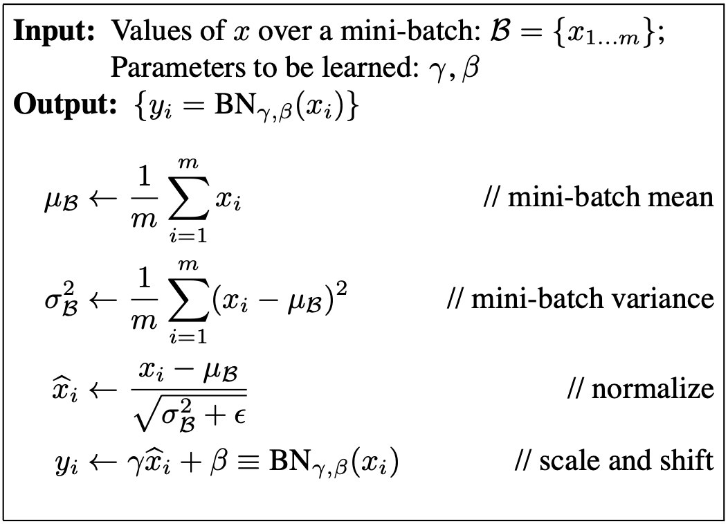
The idea is really straightforward as shown in the image below from the paper.

A bit of explanation: Taking the input mini-batch \(B = {x_1, x_2, .., x_l}\)
- We compute the mean of the mini-batch \(\mu_B\). Here it is important to notice that if the dimensions of \(B\) are \((N,D)\) with \(N\) the number of inputs and \(D\) the features of each input, we will compute the mean over \(N\) with an output of dimension \((D, )\).
- Using the mean, we compute the variance \(\sigma^{2}_{B}\). Note that the variance here is also across \(N\).
- Calculate the normalized input \(\hat x_i\). In the equation we add an epsilon term commonly set as \(\epsilon = 1e-5\) just to avoid division by zero when \(\sigma^2_B = 0\).
- Finally we add two learnable parameters \(\gamma\) and \(\beta\) that shift and scale the output. They are introduced to moderate the effect of the normalization so the net can have the same power of representation (sometimes is useful to not have zero mean and variance of 1. For example, in the case that the net doesn’t need the normalization it will learn \(\gamma=\sqrt{\sigma^2_B+\epsilon}\) and \(\beta=\frac{\mu_B}{\sqrt{\sigma^2_B+\epsilon}}\).
Implementation
The moment you were waiting for! Let’s code and start from a vanilla implementation of the forward pass for an input \(x\) of dimensions \((N, D)\) using the algorithm described above. An useful tip here is to follow up the dimensions of the transformation and the steps taken to compute the output.
def batchnorm_forward(x, gamma, beta):
  '''
  Inputs:
  - x: Data of shape (N,D)
  - gamma, beta: Scale and shift of shape (D,)
	Out:
	- out = Normalized inputs (N,D)
	- cache = Useful intermediate values
  '''
  eps = 1e-5

  #Forward pass
  mu = np.mean(x, axis=0) # mean (D,)
  var = np.var(x, axis=0) # var (D,)
  var_inv = 1 / np.sqrt(var + eps) # inverse of var (D,)
  x_mu = x - mu # input minus mean (N,D)
  x_norm = x_mu * var_inv # nomalized input (N,D)
  out = gamma * x_norm + beta # scale and shift (N,D)

  # Cache: Tupple needed for the backward pass
	cache = (gamma, x_norm, x_mu, var_inv)

  return out, cache
Backward Pass
The vanilla implementation of the forward pass can help us to build the backward pass following each step. It is a little complicated due to the mixed branches of the graph and a useful exercise is to draw the graph and use the chain rule to calculate the derivative for each node. I attached an image from the course CS231n of Stanford that shows the graph for a forward/backward pass.

In the function we will receive \(\frac{dL}{dY}\) and we will need to compute \(\frac{dL}{dX}, \frac{dL}{d\gamma}, \frac{dL}{d\beta}\) using the chain rule, \(\frac{dL}{dX}=\frac{dL}{dY}\frac{dY}{dX}\) and the intermediate values we saved in the cache variable. Again, it’s useful to follow up the change in the dimensions of the vectors to be sure that our calculations are good.
def batchnorm_backward(dout, cache):
  '''
  Inputs:
  - dout: upstream derivate
  - cache: variables for intermediate derivates
  Outputs:
  dx, dgamma, dbeta: dLoss with respect to each variable
  '''
  # Unpack cache variables
	gamma, x_norm, x_mu, var_inv = cache
  N = dout.shape[0]

  # Backward pass
  dgamma = np.sum(dout * x_norm, axis=0) # N,D -> D,
  dxnorm = dout * gamma # N,D -> N,D
  dbeta = np.sum(dout, axis=0) # N,D -> D,

  dxmu = dxnorm * var_inv  # N,D -> N,D
  dvar_inv = np.sum(dxnorm * x_mu, axis=0)  # N,D -> D,

  dvar = dvar_inv * -0.5 * var_inv ** 3 # D,
  dx = dxmu

  dxmu += dvar * 2/N * x_mu
  dmu = -1 * np.sum(dxmu, axis=0)

  dx += 1/N * dmu

  return dx, dgamma, dbeta
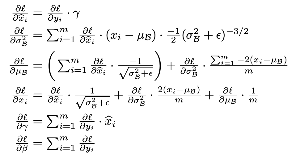
Another way to implement the backward pass is to use the numeric calculation for the derivative. After some mathematical workout you should be able to reach equations like the ones shown in the paper and in the figure below. If you are interested you can see the implementation of this function on my GitHub on this link. Implementing the backward pass using simplify gradients should be a little faster than the implementation shown above. On this notebook you can see a comparison of both where the simplify function is 13% faster.

Forward Pass: Testing Time
Although the function above for the forward pass is useful for building the backward pass, it has some flaws. In particular let’s take into account the second simplification that the authors do: the batch normalization algorithm uses the mean and variance of a mini-batch waiting that it would be representative of the input. But what happens during testing time? The input now is small, so the values won’t be representative.
To solve this we will use an exponentially decaying running mean and a running variance saved from the training time and during testing time we will normalize the inputs with these values of mean and variance. For the decaying rate we will use a momentum constant set commonly as \(\rho = 0.9\).
def batchnorm_forward(x, gamma, beta, mode):
  '''
  Inputs:
  - x: Data of shape (N,D)
  - gamma, beta: Scale and shift of shape (D,)
  - mode: train or test str
	Out:
	- out = Normalized inputs (N,D)
	- cache = Useful intermediate values
  '''
  # Unpacking the parameters	# Change btw train and test
  N, D = x.shape
	momentum = 0.9 # Setting the momentum constant

  # Initialization of mean/var for testing step
  running_mean = bn_param.get("running_mean", np.zeros(D, dtype=x.dtype))
  running_var = bn_param.get("running_var", np.zeros(D, dtype=x.dtype))

  if mode == 'train':
   	### Perform batch normalization as before

    # Adding the mean and var to the running mean
		running_mean = momentum * running_mean + (1 - momentum) * mu
		running_var = momentum * running_var + (1 - momentum) * var

		# Store the updated running means back into bn_param
    bn_param["running_mean"] = running_mean
    bn_param["running_var"] = running_var

   if mode == 'test':
    # Normalizing inputs with the saved data
    x_norm = (x - running_mean) / np.sqrt(running_var + eps)
		out = gamma * x_norm + beta

  return out, cache
You can see the complete version of this function on my GitHub account as part of my solutions for the assignment 2 of the Stanford course CS231n here.
BatchNorm Results
You may be wondering how much better it is to train a network with batch normalization and how it compares with another trained without it. As an experiment, I trained two 6-Layer Fully Connected Net on the CIFAR-10 Dataset with a batch size of 50 during 10 epochs, one with batch normalization and another without. The training loss for each of them are shown in the figure below where we can see that the model trained with batch normalization, the blue one, converges faster than one without it.

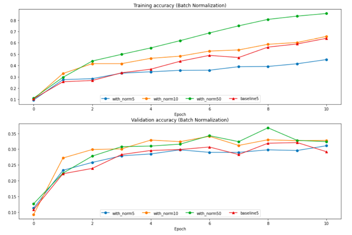
So it’s true that batch normalization improves the training of a fully connected neural net. But, the second simplification has an important side effect: what happens if the mini-batch isn’t representative of the input data? And more specifically, how does the batch size affect the representation of the data? As you can imagine, the smaller the mini-batch the less representative of the total input. In the image below you can see that four nets were trained using different batch sizes, 5, 10, 50 and no batch normalization.
We see that bigger the batch size, better the results. The problem is that in supervised learning, it’s really expensive to train over the whole training but at the time is less effective to the batch normalization to use small batches. Moreover, in networks where the mini-batches are forced to be small (online training, RNN) the results of BN are poor even compared with no BN networks (see the mini-batch of 5 samples). This is because the 𝜇 and 𝜎 of the data can’t be properly estimated and differs from the one used in BN.

Layer Normalization
Layer normalization was conceived as an intent to adresse the aforementioned problems and restrictions of BN. The paper Layer Normalization proposed to modify batch normalization and implemented the normalization across the layer instead across the mini-batch according to the following implementation:
$$ \mu_l = \frac{1}{H}\sum_{i=1}^{H}a_i^l \hspace{1cm} \sigma_l=\sqrt{\frac{1}{H}\sum_{i=1}^{H}(a_i^l-\mu_l)^2} $$
Here \(H\) denotes the number of hidden units in a layer. Here we can see that in difference to the batch normalization formulation, \(\mu_l\) and \(\sigma_l\) are shared across all the hidden layers but different training inputs will have different normalization terms. A benefit of this set up is that it doesn’t depend on the size of the inputs so layer normalization is applied in the same way when training and testing. As the authors mention “Unlike batch normalization, layer normalization does not impose any constraint on the size of a mini-batch and it can be used in the pure online regime with batch size 1.”
Implementation and Results
The implementation is really similar to batch normalization but now the statistics are caulculated across the layer. This means that if we have an input \(X\) of dimensions \((N, D)\) we will compute the mean over \(D\) having an output of dimension \((N,)\)
As the code is really similar as you can see in the block code below. In this case as before it’s a good advice to follow up the dimension of each transformation to the input.
def layernorm_forward(x, gamma, beta):
  '''
  Inputs:
  - x: Data of shape (N,D)
  - gamma, beta: Scale and shift of shape (N,)
	Out:
	- out = Normalized inputs (N,D)
	- cache = Useful intermediate values
  '''
  eps = 1e-5

  # Forward pass
  mu = np.mean(x, axis=1, keepdims=True) # mean (N,1)
  var = np.var(x, axis=1, keepdims=True) # var (N,1)
  var_inv = 1 / np.sqrt(var + eps) # inverse of var (N,1)
  x_mu = x - mu # inputs minus mean (N,D)
  x_norm = x_mu * var_inv # normalized inputs (N,D)
  out = gamma * x_norm + beta # scale and shifts (N,D)

  cache = (gamma, x_norm, x_mu, var_inv)
Using the code above, the backward pass function is an easy exercise. You can see my implementation here on my GitHub. Now let’s visualize how layer normalization behaves in practice.
In the figure above, four fully connected nets were trained using layer normalization with different batch sizes, 5, 10, 50 and no layer normalization. We can see in comparison to the nets trained using batch normalization the number of samples in the batch improves only a little the performance and the method doesn’t rely on this setting. We can see that the model trained with the smallest mini-batch performs better than the one without any normalization.
It’s important to note that this method also can have some problems if the dimension of features is small the values of 𝜇 and 𝜎 will be noisy and will not represent well the data.
Group Normalization
This recent work focuses on the fact that batch normalization performs better than layer normalization when used in convolutional neural networks. The problem is that the dependence of BN in the batch size makes it inefficient for ConvNets. We know that BN is computational expensive and since ConvNets are generally used to image recognition with high definition images usign it to train them may be not a good idea.
The authors argued that when using layer normalization all the neurons in a hidden layer have the same contribution to the final output but in ConvNets this doesn’t happen since the neurons whose receptive fields are in the border of an image are rarely turned on. They proposed a modification of the layer normalization method dividing the sample into G different groups and performing the normalization
Spatial Normalization / Spatial Group Normalization
First we will come back a little to the paper of BN to understand how to apply it to ConvNets. It’s necessary to modify a little the function since in the last one we were expecting an input \(X\) of dimensions \((N, D)\) but when working with images the input is generally of dimensions \((N, C, H, W)\) where N is the number of samples, C the channels (RBG) and \((H, W)\) the height and width of the feature map.
The following implementation shows the forward pass function for the spatial normalization. We reuse the batch normalization forward pass function changing a little the dimension of the matriz. The good question here is, which transformations must be done to a \((N,C,H,W)\) matrix to convert it to a \((N,C)\) matrix? The backward pass is analogous and you can find it here.
def spatial_batchnorm_forward(x, gamma, beta, mode):
  '''
  Inputs:
  - x: (N, C, H, W)
  - gama, beta: (C,)
  - mode: train/test
  Out:
  - out: (N, C, H, W)
  - cache
  '''
  N, C, H, W = x.shape

  # Forward pass
  x_vec = np.transpose(x, (0,2,3,1)).reshape(-1,C)	# Reshape x -> (N, C)
  out, cache  = batchnorm_forward(x_vec, gamma, beta, mode)
  out = np.transpose(np.reshape(out, (N,H,W,C)), (0,3,1,2))

  return out, cache
What the authors of group normalization proposed was to use a similar transformation to modify the layer normalization algorithm. The following code block proposes a spatial group normalization. As you can see, the function is pretty similar to the one for layer normalization but now the dimensions of the tensor are different. Again, the backward pass is straightforward but in the case you need it you can find it on my GitHub in this link.
def spatial_groupnorm_forward(x, gamma, beta):
  '''
  Inputs:
  - x: (N, C, H, W)
  - gamma, beta: (C,)
  - G: int number of groups. Should be divisor of C
  Out:
  - out: (N, C, H, W)
  - cache
  '''
  eps = 1e-5

  # Forward pass
  x_g = np.reshape(x, (x.shape[0]*G, -1))  # N*G,H*W*(C/G)
  mu = np.mean(x_g, axis=1, keepdims=True) # N*G,1
  var = np.var(x_g, axis=1, keepdims=True) # N*G,1
  var_inv = 1 / np.sqrt(var + eps) # N*G,1
  x_mu = x_g - mu # N*G,H*W*(C/G)
  x_norm = x_mu * var_inv # N*G,H*W*(C/G)
  x_norm = np.reshape(x_norm, x.shape) # (N,C,H,W)
  out = gamma * x_norm + beta

  cache = (gamma, x_norm, x_mu, var_inv)

  return out, cache
GN Performance
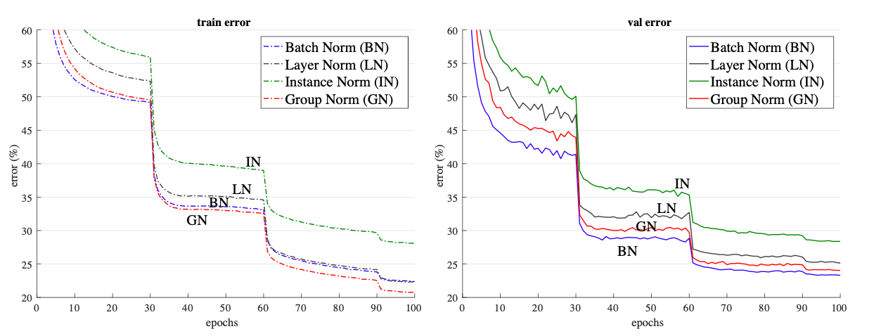
In the following figure from the paper, there are four different models’s error vs epoch curves. The models were trained each one with a normalization technique, on the right the results for the training data and on the right for the validation data. We can see that the group normalization has a better performance than all the other normalization methods while training and during validation is only outperformed by BN.

As future work, the authors proposed to see the development of this model into recurrent and generative neural networks as it’s related to layer normalization. They also mentioned that the current available models are fine-tuned to be used with batch normalization and that this can bias the results explaining the better performance of BN, so a re-design of the state-of-the-art learning systems to focus on GN may improve the results.
Conclusion
Training neural networks using SGD is a complex task. There are different ways to improve the efficiency while training these algorithms and reparametrization of the inputs has been an effective way to do it. Batch normalization makes possible faster convergences, higher learning rates and the use of saturating functions without the fear of saturation when poor initialization was done.
However, the dependency of the algorithm on the mini-batch size makes it computational expensive and inappropriate for online learning or RNNs. Layer normalization tried to face this flaw having excellent results normalizing over the hidden neurons of a layer instead over all the training batch.
Finally Group normalization, took the ideas of layer normalization and applied them to ConvNets. They segmented the units of a hidden layer in different groups and computed the normalization for each of them. The results outperformed the layer normalization techniques.
References
[1] Batch Normalization by Sergey Ioffe and Christian Szegedy
[2] Layer Normalization by Jimmy Lei Ba and Jamie Ryan Kiros and Geoffrey E. Hinton
[3] Group Normalization by Yuxin Wu and Kaiming He
[4] Deep Learning by Ian Goodfellow, and Yoshua Bengio and Aaron Courville
[5] CS231n: CNN for Visual Recognition
This post code functions are from my answers to the assigment 2 of the course CS231n.